Applying Benford's Law to Detect Election Irregularities: A Case Study on the 2020 General Election
As 2020 General Election draws to a conclusion, the losing side is, as usual, raising questions about potential election fraud. So we believe it would be interesting to see if we can use Benford’s law to detect irregularities.
Benford’s Law
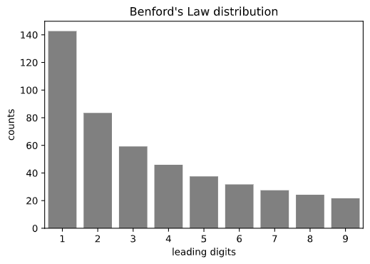
Benford’s law, or law of anomalous numbers, states that in many naturally occurring collections of numbers, the leading digit is likely to be small, with the leading digit \(d \in \{1, ..., 9\}\) occurs with probability \(P(d) = log_{10}(1 + 1/d)\). According to Wikipedia, evidences based on Benford’s law has been admitted in criminal cases at federal, state, and local levels and Benford’s law has been invoked as evidence of fraud in the 2009 Iranian election and used to analyze other election results.(1) As a caveat, there are also researches that claims using Benford’s Law is “problematic at best as a forensic tool when applied to elections”.(2) We can visualize this discrete distribution as follows:
Creating a Benford’s discrete distribution is quite straight forward in Python.
Assumption
We assume Benford’s Law distributions is the baseline expected distribution of digits occurances for fair elections. Note that this assumption is subject to controversey and there’s no theory that links this assumption to specific fraud mechanisms.(3)
Milwaukee County, Wisconsin
For the purpose of this post, we will be analyzing prescint data of Milwaukee County, Wisconsin that is published on their county website. To gather and parse the data, we used requests and BeautifulSoup4 to grab and parse the data respectively. We will be storing the data inside a dictionary of lists, with keys being names of the candidates and values being a list of precint vote counts for that candidate for ease of access.
Once we got the data, we would then preprocess them to obtain the leading digit of all of the vote counts, and count the number of occurances for each leading digits, and transform them into a dictionary of lists, with keys being names of the candidates and values being a list of leading digit counts. The preprocessing function is as follows:
Visualizations
We can then quickly visualize the expected Benford’s distribution vs observed distribution for candidates of both Democrat and Republican parties, Biden and Trump.
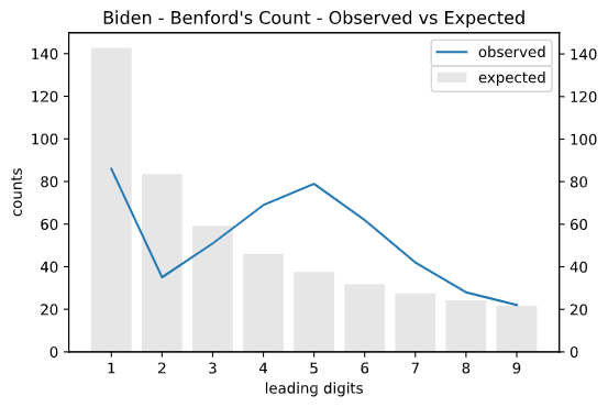
Here’s the comparison of expected vs observed Benford’s distribution for Biden. We can clearly see that Biden’s observed vs expected Benford’s distribution is visually quite different.
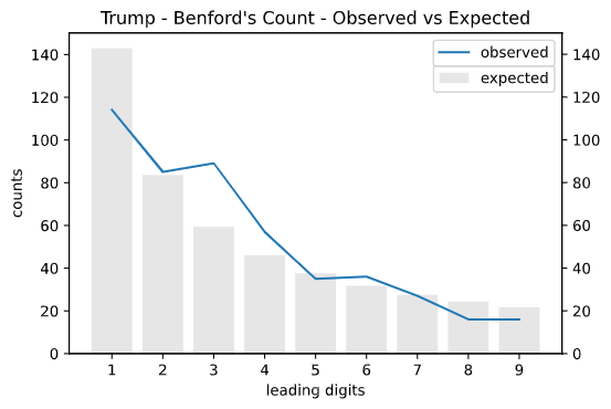
Here’s the comparison of expected vs observed Benford’s distribution for Trump. We can clearly see that Trump’s observed vs expected Benford’s distribution is visually similar.
Chi-squared Goodness of Fit test
After quick visuals, we can now conduct a statistical test to measure the goodness of fit between expected and observed data. Chi-square goodness of fit test is a non-parametric method used to compare the observed and the expected values. The expected values are based on the known theorectial distribution and in this case, Benford’s discrete distribution.
Hypothesis
Null hypothesis (\(H_0\)): There isn’t any difference between observed and the expected Benford’s distribution.
Alternate hypothesis (\(H_a\)): There is difference between observed and the expected Benford’s distribution.
Analysis Plan
We choose significance level to be 0.05.
We conduct the hypothesis testing using chi-quare goodness of fit test with scipy.stats.chisquare.
Python code to run this over our data dictionary is straightforward.
candidates = ['Biden', 'Trump', 'Blankenship', 'Jorgensen', 'Carroll']
chi_square_results = {candidate: chisquare(observed[candidate], expected[candidate]) for candidate in candidates}
Result
{
    'Biden': Power_divergenceResult(statistic=146.32065425194043, pvalue=1.1467698266391095e-27),
    'Blankenship': Power_divergenceResult(statistic=112.7312717929695, pvalue=2.4889575100879005e-21),
    'Carroll': Power_divergenceResult(statistic=93.2719008448592, pvalue=6.328417059002513e-18),
    'Jorgensen': Power_divergenceResult(statistic=14.075894069964027, pvalue=0.07980858714665816),
    'Trump': Power_divergenceResult(statistic=28.423612737925943, pvalue=0.0004000551255609517)
}
Interpretation
All of the p-values obtained from our chi-square goodness of fit test is signifncant (pvalue < 0.05) except for Jorgensen. Therefore we can reject our null hypothesis of there isn’t any difference between observed and the expected Benford’s distribution data for both Trump and Biden for the prescint election data at Milwaukee, Wisconsin.
Conclusion
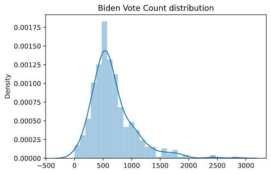
Though we are able to reject our null hypothesis, we do observe that the distribution of vote counts’ first digit for Biden is visibly different from Benford’s Law discrete distributions. One of the primary reason for that is the distribution of Biden’s prescint vote counts has a heavy peak around 500s as shown below.
We suspect the reason for that could be that the majority of the prescints could have voter registrations not exactly conforming to Benford’s Law discrete distribution thus creating a biased distribution down the line for a candidates that wins majority of the votes. Thus, our original assumption of the expected distribution conforming to Benford’s Law discrete distribution might not be valid.
Additionally, more studies could be done using Second Digits Benford’s Law technique(4), though we do note that the implied assumption of using second digit Benford’s Law is mirroring our assumption used in this study with first digit Benford’s Law.
The full code is published on Github gist.
References
2. Benford’s Law and the Detection of Election Fraud
3. Statistical detection of systematic election irregularities