Feature Selection and Dimensionality Reduction
Feature selection is an very important step in applications of machine learning methods. Modern data sets often have hundreds to thousands of features available. That is too many features for building practical machine learning models. As a data scientist and machine learning practitioner, the first step we have to do after defining the problem is to select a subset of features for model building. Or, in another sense, we will have to KonMari all the features that do not spark joy for our machine learning models and experiments.
The primary reasons for reducing the dimension of features are 1) avoid overfitting, 2) faster prediction and training, 3) smaller model and dataset, and 4) more interpretable model. This blog post is serving as a simple guide to feature selection and dimensionality reduction using Scikit-Learn.
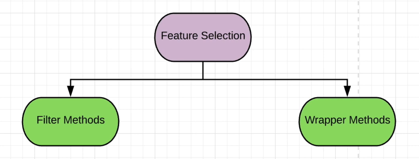
Feature selection algorithms can generally be splitted into two categories - filter methods and wrapper methods. Filter methods selects or eliminates features based on some statistical properties and tests. Wrapper methods uses some particular model, train on the dataset, and select the features based on model outputs.
Filter Methods
1. Removing Indices
We would first eliminate indexing and primary-key features, e.g., uid, user_uid, click_uid, etc. These features usually have extremely high cardinality, not continuous, and do not contain enough information related to the target variable.
However, we note that the datetime and/or timestamp features can be very useful in engineering new feature sets. For example, we can extract features such as month, days_of_week, week, and day from datetime and timestamp indices. This information could be particularly useful for time-series problems.
2. Removing Features with a High Percentage of Missing Values
The second sets of features we should be removing are the features with a high percentage of missing values. This is an unsupervised approach. The reason we want to filter them out is that it might be difficult to find the optimal method of filling the null values. For example, we can impute NaNs using mean or median, or impute using model-driven imputation with another model, or use MICE in the fancyimpute package. These methods bring extra complication and introduce potential modeling biases into the downstream feature selection process.
We can filter out the high percentage of missing value features using Pandas:
# set min NaN threshold at 20%
nan_threshold = 0.2
nan_percent = df.isna().mean()
df = df.loc[:, nan_percent <= nan_threshold]
NOTE: In addition to removing features with high percentage NaNs, we can at the same time engineer new features for each of the features removed. We can set the values to True if the value is not NaN and False if the value is NaN. For example,
# Creating a Pandas DataFrame of randomly placed missing values in with 4 columns, 'A', 'B', 'C', 'D'.
M, N, c = 20, 4, 5
A = np.random.randn(M, N)
A.ravel()[np.random.choice(A.size, c, replace=False)] = np.NaN
df = pd.DataFrame(A, columns=['a', 'b', 'c', 'd'])

# Engineer a new feature for 'd' that flags if 'd' is null.
df['feature_d_isna'] = df['d'].isna()
3. Removing Features with Low Variances
Another unsupervised approach for feature selection and dimensionality reduction is filtering out features with low variances. Generally speaking, there are two types of low variance features:
- Zero-variance (constant value) features. We can quickly filter them out with Pandas:
non_unique_columns = df.columns[df.nunique() > 1] df = df[non_unique_columns] - Low variance features. Scikit-learn provides a module named
VarianceThresholdto eliminate features using a variance threshold.
We can model features with only two values (excluding NaN) as Bernoulli random variable. Thus the variance of them is given by \(Var[X] = p(1-p)\) We can then set the threshold percentage p to remove features without sufficient variance.
Alternatively, we can remove features assuming that they are normally distributed. However, it will be prudent to verify that the features are Gausssian random variables before making the assumption. Some of the naturally observed variables will have to be log-transformed to turn into Gaussians. The following code snippet shows how to remove low variance binary features using Scikit-Learn VarianceThreshold module.
from sklearn.feature_selection import VarianceThreshold

variance_threshold = 0.8
vt = VarianceThreshold(threshold=(variance_threshold * (1 - variance_threshold)))

# Get the mask for selecting the feature columns
low_var_col_mask = vt.fit(X_binary).get_support()

# find the selected feature columns
X_binary_new = X_binary.loc[:, low_var_col_mask]

# store the list of removed features for future reference
features_removed = list(set(X_binary.columns) - set(X_binary_new.columns))

print(f"Num features removed: {np.sum(~np.array(low_var_col_mask))}")
4. Covariance-based
We can also filter out features that are highly correlated with each other. This is another unsupervised approach. This method is great for low-dimensional data. We can conduct covariance selection as following using Scipy and Scikit-Learn:
from sklearn.preprocessing import scale
from scipy.cluster import hierarchy

# Assuming feature X and target y
X_scaled = scale(X)

# Calculate covariance matrix
cov = np.cov(X, rowvar=False)

order = np.array(
    hierarchy.dendorgram(
        hierarchy.ward(cov,
        no_plot=True
    )['ivl'], dtype='int'
    )
)
5. Feature Selection using ANOVA F-Score
Another choice that we have in filtering down the number of features is to run based on supervised univariate statistical test to select the top K variables or percentile of variables based on F-test estimate the degree of linear dependency between two random variables. The following is a quick example for calculating F-scores of features for a classification task and generate a Pandas dataframe of features and their respective scores.
from sklearn.feature_selection import SelectPercentile, f_classif

sp = SelectPercentile(f_classif, percentile=10)
f_classif_mask = sp.fit(X_notnull, y).get_support()
df_f_scores = pd.DataFrame({"feature": X_notnull.columns, "f_score": sp.scores_})
Note: The selector can be f_classif or mutual_info_classif for classification or f_regression and mutual_info_regression for regression. There’s also chi1 for classification but, as usual, it requires the features to be greater than 0 otherwise it will throw errors for taking log of 0!
6. Feature Selection using Mutual Information
An alternate way of selecting features is using supervised univariate mutual_info_classif. This is a non-parametric method and we found it more helpful than ANOVA F-Score for most datasets.
Mutual information is a way of summarizing how much knowing one random variable X tells you about another random variable Y. If X and Y are independent, then mutual information is zero. Any correlation, positive or negative, will result in positive mutual information. Mutual information can be expressed in terms of Entropy (\(H\)):
\[MI(X, Y) = H(X) + H(Y) - H(X, Y)\]Note that mutual information is not predictability, i.e. \(p(X, Y)\).
from sklearn.feature_selection import SelectPercentile, mutual_info_classif

sp_mutual_info = SelectPercentile(mutual_info_classif, percentile=10)
mutual_info_classif_mask = sp_mutual_info.fit(X_notnull, y).get_support()
df_mutual_info = pd.DataFrame({"feature": X_notnull.columns, "mutual_info": sp_mutual_info.scores_})
Wrapper Based
1. Model-Based Feature Selection
Another way of selecting features is directly selecting using feature importances from some easily calculated regressors or classifiers. This is a supervised model-based approach. It uses either L1-distance2 or tree-based feature importances. Here, we are using ExtraTreeClassifier from Scikit-Learn package. Note that in our experiences, tree-based feature selection is not compute intensive, but Lasso or L1-distance based feature selection tends to take a long time as the number of features increases.
from sklearn.ensemble import ExtraTreesClassifier
from sklearn.feature_selection import SelectFromModel

etc = ExtraTreesClassifier()
etc = etc.fit(X, y)
sfm = SelectFromModel(etc, prefit=False)
X_sfm = sfm.fit(X, y)
df_sfm_etc = pd.DataFrame({"feature": X.columns, "sfm_etc": sfm.estimator.feature_importances_})
sfm_threshold = sfm.threshold_
2. Recursive Feature Elimination
We can also utilize iterative model-based approaches in selecting features. This idea can be implemented in backward: fit model, find the least important feature, remove, and iterate, or forward start with a single feature, find the most important feature, add, and iterate.
Here, we will present the Recursive Feature Elimination algorithm 3 for selecting features. RFECV is implemented within Scikit-Learn library. The recursive feature elimination algorithm starts with all the features, and iteratively removes step number of features by feature importances or coefficients, and iterate with cross-validation. The expected runtime is:
The run time of using RFECV will be much longer than any of the previous methods mentioned due to the number of fits required for this algorithm to converge.
etc = ExtraTreesClassifier()

# Minimum number of features to consider
min_features_to_select = 10
rfecv_null = RFECV(estimator=etc, step=3, cv=StratifiedKFold(2),
              scoring='f1', n_jobs=-1,
              min_features_to_select=min_features_to_select)
rfecv_null.fit(X_null_dropna, y_dropna)
print("Optimal number of features : %d" % rfecv_null.n_features_)

# Create dataframe of which features are picked by the algorithm
df_rfe_null = pd.DataFrame({"feature": X_null_dropna.columns, "rfe": rfecv_null.support_})
NOTE: .support_ attribute contains the boolean mask for the selected features, and .rank_ contains the ranks of the features, with all selected features as integer 1.
3. Forward and Backward Feature Selection
New with Scikit-Learn 0.24, it now has a forward feature selection algorithm implemented with SequentialFeatureSelector. The SequentialFeatureSelector is an iterative model-based approach that can be applied with ANY model. This algorithm shrinks/grows the feature set by greedy search and can operate in ‘forward’ mode, which slowly adds a feature at a time until the number of features converges to n_features_to_select with the highest score. The algorithm can also operate in ‘backward’ mode, which slowly removes features until convergence. The expected runtime is:
References:
2. Linear Model Selection and Regularization