Tuning XGBoost Parameters

Gradient boosting is one of the most powerful techniques for applied machine learning and has been one of the top algorithms in Kaggle competitions. In this post we are going to cover how we tuned Python’s XGBoost gradient boosting library for better results.

There are many hyper parameters in XGBoost. Below here are the key parameters and their defaults for XGBoost.

• learning_rate=0.1 (or eta. shrinkage)
• n_estimators=100 (number of trees)
• max_depth=3 (depth of trees)
• min_samples_split=2
• min_samples_leaf=1
• subsample=1.0

Tuning of these many hyper parameters has turn the problem into a search problem with goal of minimizing loss function of choice. With XGBoost, the search space is huge. Imagine brute forcing hyperparameters sweep using scikit-learn’s GridSearchCV, across 5 values for each of the 6 parameters, with 5-fold cross validation. That would be a total of 5^7 or 78125 fits!!! Even at one minute per fit, that will take over 54 days to sweep those hyper parameters. Thus, we must apply some engineering processes, heuristic, and judgment to narrow down the search space. And pray we don’t land in a local minima.

We will use the Tanzania Water Pumps data set. It is a multi-class classification data set so we will use merror and mlogloss as our evaluation metric. We will plot the training and validation merror and mlogloss vs. number of epoch during the fitting process.

Train/Validation Loss Curve

For small data sets, the default n_estimators=100 is a good start. Since this data set is of a decent size, we will set the number of trees to be 1000. The initial search space of the data set is 2,376,000. Here are our merror and mlogloss vs epoch.

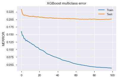
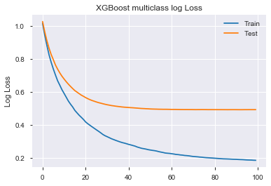
One key ‘feature’ of XGBoost is that the training error will continue to decrease and eventually overfit perfectly even as validation errors plateaued and start to invert. This small fit job took us 95 epochs. As a general rule of thumb, we can now set early_stopping_rounds to 1/10 of that or less. early_stopping_rounds will stop the training process after it see that number of rounds without improvement in validation error. Also, if multiple eval_metrics are used, it will use the last metric on the list to determine early stopping. The test accuracy of 80.6% is already better than our base-line logistic regression accuracy of 75.5%.

Sampling GridSearchCV

With early stopping set, we can try to do a brute force grid search in a small sample space of hyper parameters. It has to be noted that increases in n_estimators, max_depth and decreases in learning_rate will all increase the training time significantly. For example, fitting the data without cross validation, n_estimators=100, max_depth=20, learning_rate=0.1 takes about 1:30 minutes. But if we fit n_estimators=1000, max_depth=15, lr=0.03, it will take a whooping 10:05 minutes.

We decide to sweep max_depth=[3, 6, 9, 12], n_estimators=[600, 900, 1200, 1500], and learning_rate=[0.003, 0.01, 0.03] with what we have on our previous trial run. For sanity’s sake, we will set grid search’s cross validation to 3-Fold to reduce the training time. That will be a total of 4 x 4 x 4 x 3, or 144 fits. At an average of 5 minutes per fit, that will take around 720 minutes.

After the grid search finished training in 11 hours, the best parameters found was learning_rate=0.03, max_depth=12 and n_estimators=900. We will pull all of the mean_test_score, std_test_core, and params out of GridSearchCV and see how they vary.

means = model.cv_results_['mean_test_score']
stds = model.cv_results_['std_test_score']
params = model.cv_results_['params']
for mean, stdev, param in zip(means, stds, params):
    print("%f (%f) with: %r" % (mean, stdev, param))

Looking at the accuracy scores and the standard deviation of the accuracy scores, we see a big step up when n_estimators increase to 900 from 600 and the subsequent increases do not have as much of an impact. This coincides with our initial guesstimate of 1,000. Also, at around 900, the score standard deviation is usually the lowest.
Moreover, the table also showed that we need deeper trees, since at max_depth=12, the training score is still lower than our initial guesstimate of max_depth=20. Our guts tells us we should stay around 20 for max_depth. Since we are building deeper trees, we decide to adjust the learning rate to 0.01 instead of the best parameter 0.03. It should help against over fitting.

Narrower Search

Now, we will fit from what we’ve learned from the prior training and grid search. We will use max_depth=20, n_estimators=800, learning_rate=0.01, and train using 5-fold cross validation. The fitting process takes around 30 minutes and we achieve a validation score of 82.05%.

To verify that we are close to a minima, we conducted another grid search, sweeping around current best parameters, with max_depth=[18, 20, 22, 24] and n_estimators=[900, 1050, 1300, 1450].

The fitting process took 288 minutes and yielded the best parameter of max_depth=18 and n_estimators=1050, with accuracy score exactly the same as our last set of parameters. We have found the local minima.

Here’s our abridged progress history:

• logistic regression baseline: 75.5%
• XGBoost Guesstimate v1: 80.2%
• XGBoost GridSearchCV Wide: 80.7%
• XGBoost Guesstimate v2: 82.0%
• XGBoost GridSearchCV Narrow: 82.0%

Visualization

XGBoost library includes a few nifty methods for visualization.

We can use the plot_tree method to visualize one of the trees in the forest. Due to the depth of our trees, the output tree visualization became too hard to read.

from xgboost import plot_tree

fig, ax = plt.subplots()
xgboost.plot_tree(model, num_trees=1, ax=ax, rankdir='LR')
plt.show()

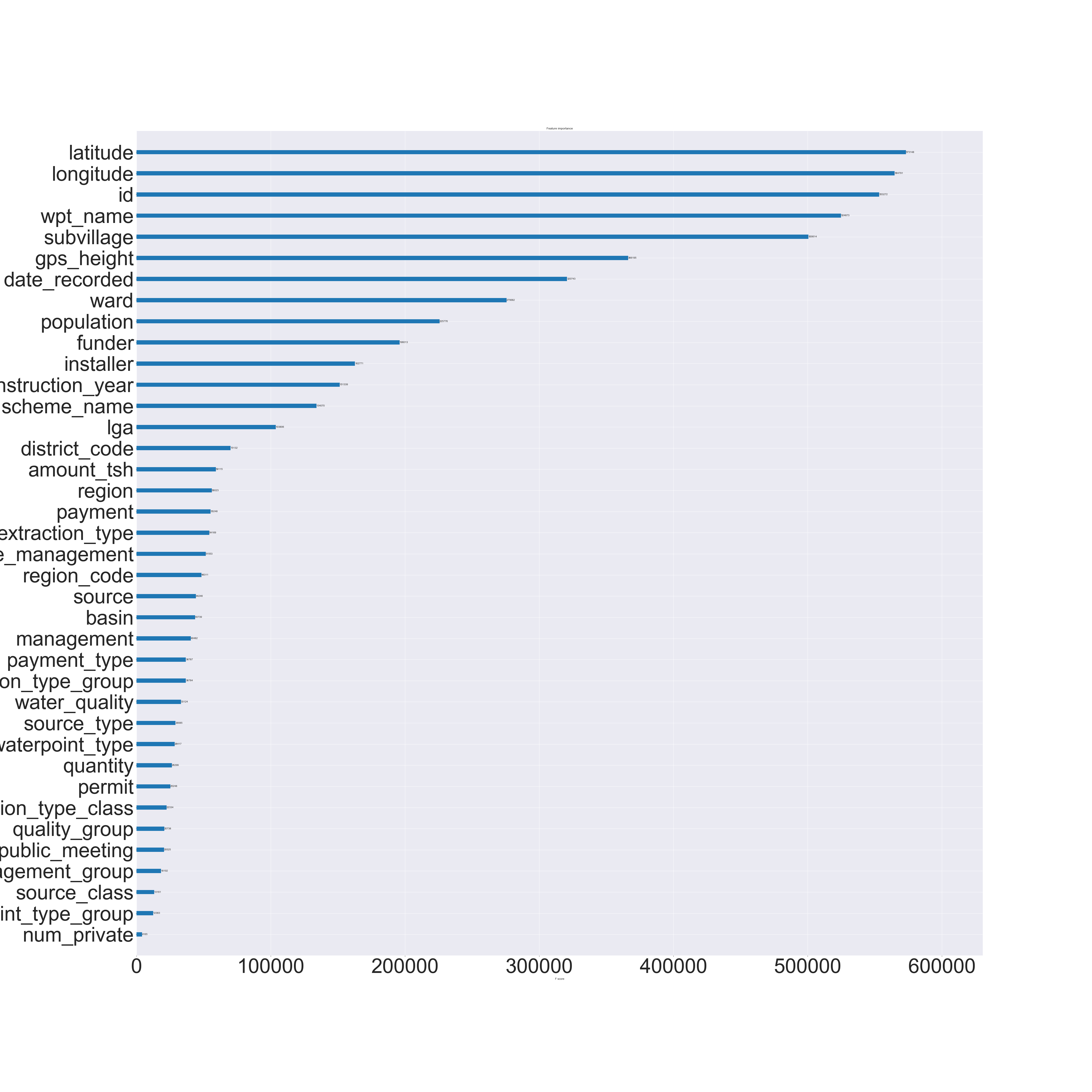
Or, we can use plot_importance to plot a horizontal bar chart of feature importances. Here’s a quick code block and the plot for our data set.

from xgboost import plot_importance

fig, ax = plt.subplots()
plot_importance(model, ax=ax)
plt.show()

Conclusion

Here’s our pseudocode for the hyperparameter tuning process. This an zero’th order optimization w/ adaptive selection with human level adaptive search.

While search(params).best != train(guess_params).best
  guess_param <- educated guess
  train(guess_param)

  params <- spaces around educated guess
  grid/randomized search(params)

  if search(params).best > train(guess_param).best
    guess_param <- params.best

  repeat until search(params).best = train(guess_param).best

We were unfortunate to sweep the wrong regions of the hyper parameter search space during our half-day-long grid searching. Perhaps we could cover a wider sweep using randomized search, or even better, utilize Auto-ML libraries such as TPOT, auto-sklearn, H2O or Google’s AutoML to make life better.

Looking back, one improvement we could have done is apply randomized sampling during the searching process so we could speed up the search.

Hyper parameter tuning is a search problem and these reinforcement learning based AutoML libraries can and should do better than humans in general. But the question is, how would we build domain expertise then?

---

To cite this content, please use:

@article{
    leehanchung,
    author = {Lee, Hanchung},
    title = {Tuning XGBoost Parameters},
    year = {2019},
    howpublished = {\url{https://leehanchung.github.io}},
    url = {https://leehanchung.github.io/xgboost/}
}