Agents Are Workflows
AI agents perceives its environment, make sequential decisions, and take actions to achieve specific goals as measured by the rewards. LLM based AI agents are no exception.
A powerful way to interpret and operationalize these agents is by unrolling their decision-making processes into structured representations like Directed Acyclic Graphs (DAG) or Finite State Machines (FSM). This blog post provides grounding on how we can achieve this and why this is true by leveraging Bellman’s Equation, a cornerstone of reinforcement learning (RL). We’ll formulate our LLM based AI agents using Bellman’s Equation and provide derivations on unrolling AI agents into DAGs and FSMs.
Modeling LLM Agents
The defining characteristic of LLM agents is that they operation in a sequential decision making loop. At each step, the agent:
- Observes its current state based on environmental input and its internal memory including chat history.
- Thinks using its internal latent state or with
<thinking></thinking>for the reasoning models to determine the best action towards its goal. This is thepolicy, the strategy for selecting actions based on states. - Acts by generating text, calling a tool, or executing a command.
This cycle repeats, with the agent updating its chat history priors and make decisions based on the outcomes of its actions. This sequential state, action, and objective behavior over time is the perfect fit for Markov Decision Processes (MDP) to modeling these agents.
Markov Decision Process and Bellman’s Equation
Markov Decision Process (MDP)
An MDP provides a structured way to model problems where an agent learns to achieve a goal through trial-and-error interactions with an environment.
An MDP is formally defined as a tuple M=⟨S,A,T,R,γ⟩, where :
- $S$: A finite set of possible states. In the context of an LLM agent, a state $s\in S$ encapsulates all relevant information at a given time step, including the conversation history, retrieved documents, internal memory contents, and observations from the environment.
- $A$: A finite set of possible actions. For an LLM agent, an action $a\in A$ could be generating a text response, thinking, or using a tool (via API or MCP).
- $T(s^\prime∣s,a)=P(s_{t+1} = s^\prime ∣ s_t =s,a_t =a)$: The transition probability function. This is the probability of transitioning to state $s^\prime$ at the next time step, given that the agent is currently in state $s$ and takes action $a$. This captures the dynamics of the environment and the effects of the agent’s actions.
- $R(s,a,s^\prime)$: The reward function. This defines the immediate reward $r_{t+1}$ received by the agent after transitioning from state $s$ to state $s^\prime$ by taking action a. Rewards provide feedback signal to guide agent towards its goal.
- $\gamma$: The discount factor $(0\leq \gamma \leq 1)$ that determines the present value of future rewards. A value close to 0 prioritizes immediate rewards, and close to 1 emphasizes long-term rewards.
A key assumption underlying MDPs is the Markov Property: the transition probability $T(s^\prime∣s,a)$ and immediate reward $R(s,a,s^\prime)$ depend only on the current state $s$ and action $a$, not on the entire history of previous states and actions. For LLM agents, this implies that the defined state representation, including chat history and memory, must sufficiently summarize the past to predict the future.
Value Functions
The goal of an agent in an MDP is to maximize the expected cumulative discounted reward over time. To achieve this, we define value functions that quantify the long-term desirability of states or state-action pairs under a given policy $\pi(a \vert s)$. A policy defines the probability of taking action $a$ in state $s$. We define values by value of the state or value of the action.
Note: LLM itself and its thought process IS the policy $\pi$.
State Value Function ($V^{\pi}(s)$): The expected cumulative discounted reward starting from state $s$ and subsequently following policy $\pi$, or $V^{\pi}(s) = \mathbb{E}_{\pi}$. This tells us “how good” it is to be in state s under policy $\pi$
Action Value Function ($Q^{\pi}(s,a)$): Or the Q-function to distinguish from $V$ state value function notation. The expected cumulative discounted reward starting from state $s$, taking action $a$, and subsequently following policy $\pi$, or $Q^\pi(s, a) = \mathbb{E}_\pi$. This tells us “how good” it is to take action a in state $s$ and then follow policy $\pi$.
Bellman’s Equation
The Bellman equation, named after Richard Bellman, is a recursive formulation used to compute the optimal value of a state in an MDP. It expresses the value of a state as the expected reward for taking an action plus the discounted value of the next state. For a state $s$, action $a$, reward $r$, next state $s^\prime$, discount factor $\gamma$, and value function $V$. Assume the optimal policy $\pi^*$ that selects the actions that maximizes the expect return. The Bellman’s Equation for $v^\pi$ is:
\[v^\pi(s) = \sum_{a}\pi(s,a) \sum_{s^\prime}p(s^\prime, r\vert s,a) [r + \gamma v^\pi(s')]\]where:
- $p(s^\prime, r \vert s, a)$: Transition probability to state $s^\prime$ with reward $r$ from state $s$ given action $a$
- $r$: reward
- $\gamma$: Discount factor $0 \leq \gamma < 1$, balancing immediate vs. future rewards.
- $v^\pi(s’)$: Value of state $s$ following the policy $\pi$.
Or, if we simplify it to its raw form, the value function of a state is the reward of the current state plus the discount reward of its future state, or,
\[v_\pi(s) = \mathop{\mathbb{E}}[r(s, a) + \gamma v_\pi(s^\prime)]\]The Bellman equation’s recursive nature explicitly linking the value at one step, $V(s)$ or $Q(s,a)$, to the value at the next step $V(s′)$ or $Q(s′,a’)$. It models the temporal dependency inherent in sequential decision-making. This structure, where value computation progresses iteratively or recursively through time, forms the basis for representing the process as a Directed Acyclic Graph (DAG). Reinforcement Learning algorithms like Value Iteration or Policy Iteration directly implement this recursive update, making the connection to DAGs explicit.
Unrolling LLM Agents
Agent as DAG
Directed Acyclic Graphs (DAGs) are mathematical structures consisting of nodes (vertices) and directed edges, with the crucial property that there are no directed cycles. This means one cannot start at a node, follow a sequence of directed edges, and return to the starting node. DAGs are widely used to model processes with dependencies, such as task scheduling in workflow orchestration tools (e.g., Apache Airflow, Argo Workflows), data processing pipelines (e.g., Apache Spark), and computational dependencies. The directed edges enforce a logical execution order based on dependencies.
Recall value function:
\[v^\pi(s) = \mathop{\mathbb{E}}[r(s, a) + \gamma v_\pi(s^\prime)]\]its recursion encapsulated all future behaviors of an agent in a single self reference. Each successive substitution of the right hand side into the remaining $v_\pi$ term unrolls the horizon further out:
\[v^\pi(s) = \mathop{\mathbb{E}}[r_0 + \gamma r_1 + \gamma^2 r_2 + \cdots + \gamma^{k-1}r_{k-1} + \gamma^k r_k)]\]We can define the DAG $\mathcal{G}_{DAG}$ representing the Bellmans unrolling:
- Nodes ($\mathcal{N}$): Each node represents the value of a specific state $s\in S$ at a specific timestamp $t$. Let a node be denoted as $(s,t)$. We typically consider iterations k=0,1,…,K for some maximum iteration count K. So, N={(s,k)∣s∈S,0≤k≤K}.
- Edges ($\mathcal{E}$): A directed edge exists from node $(s′,k)$ to node $(s,k+1)$ if the value $v_t(s′)$ contributes to the calculation of $v_{t+1}(s)$ via the Bellman equation. Specifically, an edge $((s′ ,k),(s,k+1))$ exists if there is at least one action $a\in A$ such that the transition probability $p(s′∣s,a)>0$.
- Structure: The DAG is layered by timestamp $t$. Edges only go from layer $t$ to layer $t+1$. Because the computation proceeds forward in iterations (or backward in time for finite horizon), there are no cycles, satisfying the acyclic property of DAGs
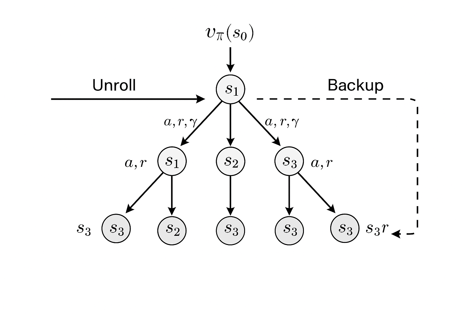
Conceptualy, every subsitution of unrolling Bellman’s adds a new layer of successor states. Treat each state and timestamp pair $(s, t)$ as a node and each policy probablistic transition $(s_t, a_t, r_t) \rightarrow (s_{t+1}, t+1)$ as a directed edge. The repeated states across branches coalesces into the same vertex.
The root node is the current state, leaves are either the terminal states or the state where we stop unrolling. Because time only advances, edges never point backward, so the structure obtained here is a direct acyclic graph rather than a cyclic MDP.
Agent as FSM
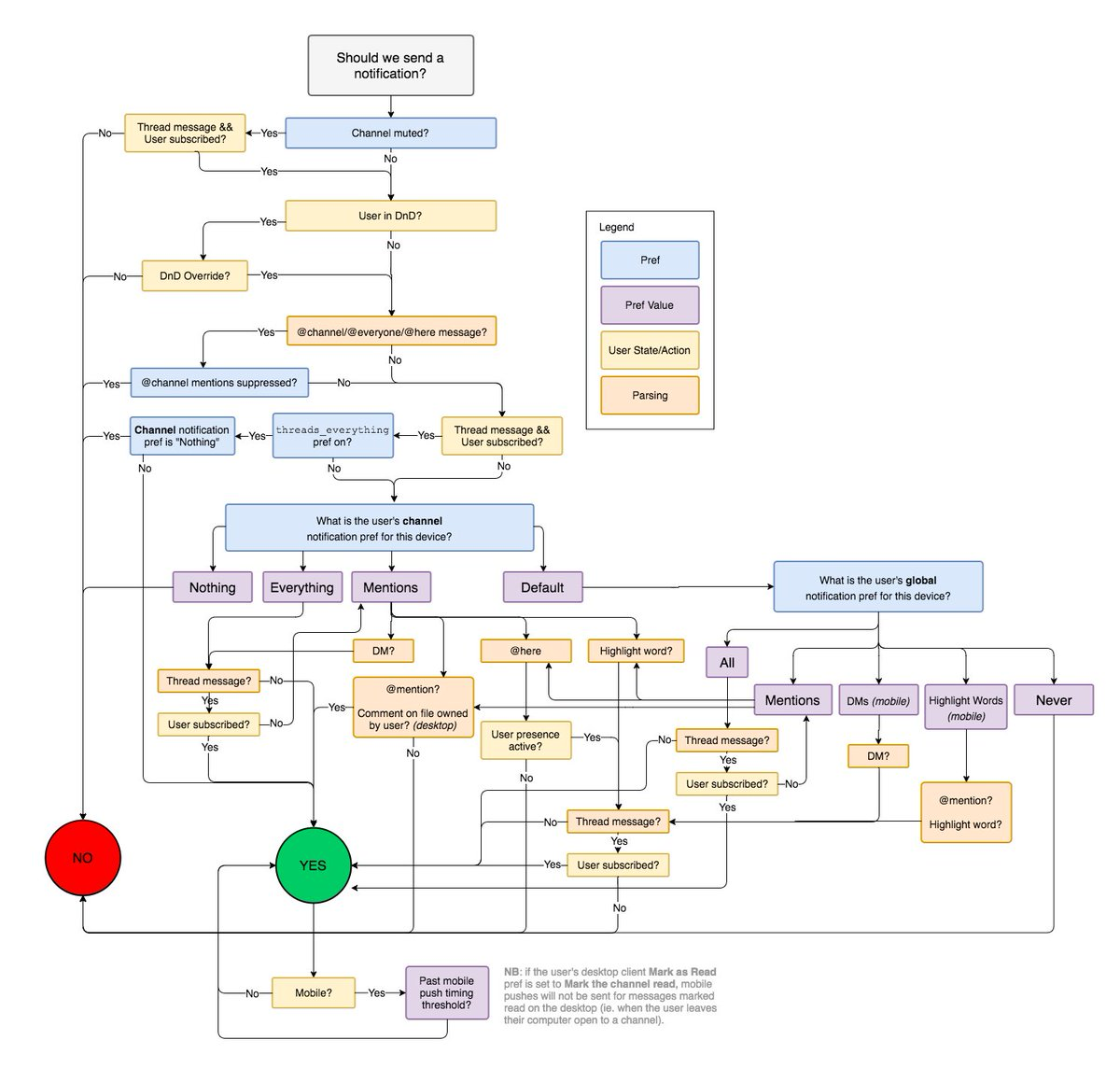
Finite State Machines (FSMs), also known as Finite Automata (FSA), are fundamental models of computation used to describe systems that can be in one of a finite number of states at any given time. An FSM transitions between these states based on inputs it receives. FSMs can be used as acceptors (recognizing sequences), classifiers, transducers (producing outputs based on inputs/states), or sequencers. Example of FSM includes vending machines, Slack notification logic, or Claude Code.
Representing an LLM agent as an finite state machine is more challenging. The state space of an agent, including conversation history, memory, and its external environments is likely huge or practically infinite. Since FSMs require a finite number of states by definition, a direct mapping is generally intractable.
Thus, we will take the standard approach to handle large state spaces with state aggregation, or node agglomeration. The core idea is to partition the original large state space $S$ into a smaller, finite number of disjoint subsets as aggregated states. Each aggregate state groups together original states that are considered “similar” according to some criterion. This process of grouping nodes is precisely the “node agglomeration” required to construct a tractable FSM from the underlying MDP model of the agent.
The Bellman equation provides measure of state value and actions offers criteria for defining state similarity and performing aggregation. Other criterias exist, such as grouping states with similar transition probabilities or reward structures.
Using state aggregation, we can define an FSM $M_{FSM}=⟨Q_{FSM},\sum_{FSM}, \delta_{FSM}, q_0⟩$ that approximates the behavior of the agent described by the original MDP $M=⟨S,A,T,R,\gamma⟩$:
- FSM States (Q_{FSM}): A finite set of aggregate states. Each $q \in Q_{FSM}$ corresponds to a subset of the original MDP states $S_q \supseteq S$. The partitioning is defined by an aggregation function $\mathbb{\Phi}: S\rightarrow Q_{FSM}$, The aggregation function $\mathbb{\Phi}$ is constructed based on the chosen criterion such as similarity of $V_∗(s)$ or equality of $\pi_∗(s)$.
- FSM Alphabet ($\sum_{FSM}$): The set of inputs that trigger transitions in the FSM. These might correspond directly to the MDP actions $A$, or they could be more abstract events or observations derived from the environment.
- FSM Transition Function ($\delta_{FSM}$): $\delta_{FSM}: Q_{FSM} \times \Sigma_{FSM} \rightarrow \Delta(Q_{FSM})$ for probabilistic FSMs, where $\Delta(Q_{FSM}$ is the set of probability distributions over $Q_{FSM}$. Defining $\delta_{FSM}$ requires summarizing the underlying MDP transitions $P(s′∣s,a)$ for all $s \in S_q$ with approximation, e.g. averaging transition probabilities or weighted sums based on state distributions. This leads to some loss of information vs the original MDP.
- FSM Initial State ($q_0$): The aggregated FSM state that contains the initial state($s$) of the MDP.
The FSM derived through state aggregation or node agglomeration provides a high-level, abstract model of the LLM agent’s behavior. It provides a more interpretable representation of the agent’s aoperational modes with some sacrifices on the fine-grained detail of the original MDP. This models is valuable for understanding the overall structure of the agent’s strategy, identifying stable behavioral regimes, or even designing high-level controllers or monitors for the agent.
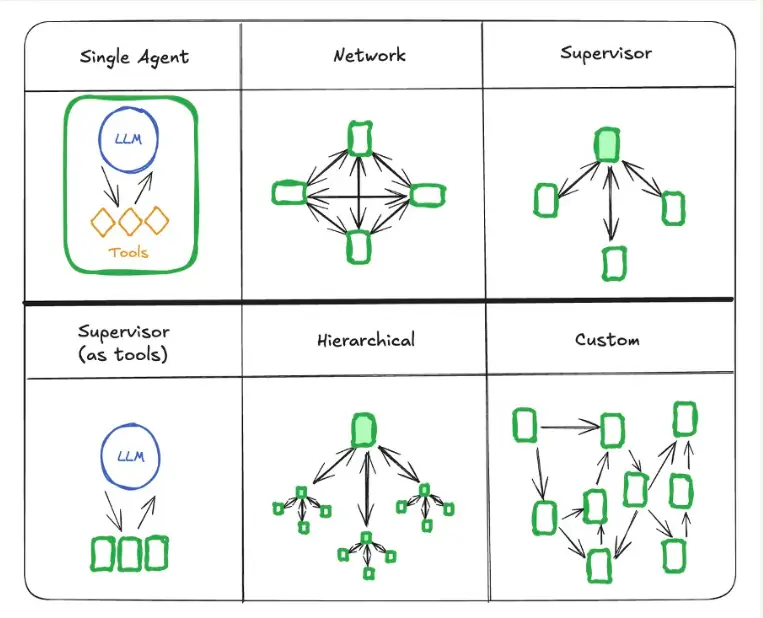
Actually, the application developers have already unconsciously been doing node agglomeration to break down and approximate a complex agent into various different finite state machines and call them “design patterns”.
Comparison Table
The following table summarizes the key differences between the DAG and FSM representations derived from the Bellman equation:
| Feature | DAG Representation (Bellman Unrolling) | FSM Representation (State Aggregation) |
|---|---|---|
| Representation Focus | Computational flow of value determination | Abstract behavioral modes / policy structure |
| Granularity | Detailed step-by-step value dependencies | High-level aggregated states |
| State Space | Explicitly represents values for all states at each step | Represents a drastically reduced set of abstract states |
| Cycles | Acyclic by definition | Can contain cycles representing recurring behaviors |
| Derivation | Direct unrolling of Bellman equation | Bellman values/policy + State Aggregation + Transition Approximation |
Conclusion
We have explored two distinct pathways for transforming the sequential decision making process of an LLM agent, modeled as an MDP and analyzed via the Bellman equation, into computational structures: DAGs and FSMs.
- DAG via Unrolling: Leverages the recursive structure of the Bellman equation itself. The equation defines how values at one timestep or iteration depend on values at the previous iteration (or next timestep). Unrolling this recursion directly maps the computational dependencies into a layered, acyclic graph.
- FSM via Aggregation: Uses the Bellman equation as a basis for simplifying the system. States with similar values or identical optimal actions are grouped into aggregate states, forming the basis of a finite state machine.
These provide structured ways to understand and design complex agentic systems. Further, they help in verification and debugging, helping to identify potential inconsistencies or failure modes in the agents.
References
- Sutton, R. S., & Barto, A. G. (2018). Reinforcement learning: An introduction (2nd ed.). MIT Press.
- Bellman, R. (1957). A Markovian Decision Process. J. of Mathematics and Mechanics.
@article{
    leehanchung,
    author = {Lee, Hanchung},
    title = {Agents Are Workflows},
    year = {2025},
    month = {05},
    howpublished = {\url{https://leehanchung.github.io}},
    url = {https://leehanchung.github.io/blogs/2025/05/09/agent-is-workflow/}
}